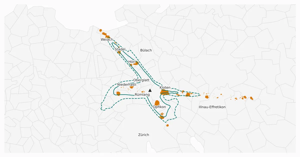
Live Flight Data Step by Step - Part 12 - Who is overflown?

So far, the flights have been the subject of this series. This part looks at the ground instead: where are aircraft low, and who lives there?

The data is the same as in parts 4 to 9 and 11: the Swiss feed from 20 October, 14:00 to 21 October, 11:59 Swiss time. That’s a Tuesday afternoon, one night and a Wednesday morning. Everything that follows describes those 22 hours, not a typical year.

Three new data sets come from outside, all open:

• the municipality boundaries of the Federal Statistical Office (BFS), as of 1 January 2025
• the population: per municipality (31 December 2025) and per hectare (2024), both from the BFS population statistics STATPOP
• the official noise contours of Zurich airport from the noise exposure cadastre of the Federal Office of Civil Aviation (BAZL), via the WFS of the Canton of Zurich

Where the ground data comes from

All three are downloaded once by the notebook and kept in a local cache/ folder. A small helper, fl.cached(url, filename, max_age_days), downloads a file only if it’s missing or older than the given number of days.

Municipality boundaries. The BFS publishes the generalised municipality boundaries as one zip file (about 11 MB) with several versions inside. I take one GeoJSON from it: the historised boundaries as of 1 January 2025, in the K4 level of detail and in WGS84 coordinates.

GG25_URL = "https://dam-api.bfs.admin.ch/hub/api/dam/assets/34367751/master"
GG25_MEMBER = ("ag-b-00.03-875-gg25/Historized boundaries K4 20250101/"
               "Communes_K4_20250101_4326.geojson")
geojson = zipfile.ZipFile(fl.cached(GG25_URL, "gg25.zip", 365)).read(GG25_MEMBER)

That gives 2,121 polygons. Besides the BFS number (GDENR) and the name, each one carries the area and elevation statistics – the mean elevation Z_AVG is used in the next section.

Population per municipality. STATPOP, the population statistics of the BFS, are available as table px-x-0102010000_101 through the PXWeb API. The query asks for the year 2025, all municipalities and the permanent resident population, with nationality, sex and age each set to “total”:

url = "https://www.pxweb.bfs.admin.ch/api/v1/de/px-x-0102010000_101/px-x-0102010000_101.px"
query = {"query": [
    {"code": "Jahr", "selection": {"filter": "item", "values": ["2025"]}},
    {"code": "Kanton (-) / Bezirk (>>) / Gemeinde (......)", "selection": {"filter": "all", "values": ["*"]}},
    {"code": "Bevölkerungstyp", "selection": {"filter": "item", "values": ["1"]}},
    {"code": "Staatsangehörigkeit (Kategorie)", "selection": {"filter": "item", "values": ["-99999"]}},
    {"code": "Geschlecht", "selection": {"filter": "item", "values": ["-99999"]}},
    {"code": "Alter", "selection": {"filter": "item", "values": ["-99999"]}},
], "response": {"format": "csv"}}

The answer is a CSV in Latin-1 that mixes cantons, districts and municipalities in one column. Municipality rows start with six dots, like ......0261 Zürich, so the regex ^\.{6}(\d{4}) (.*) picks them out. Each request took about 30 seconds, so I ran it once and saved the result as a small CSV in the repository: 2,115 municipalities, 9,127,125 people, Zurich 440,935.

Population per hectare. The BFS also publishes STATPOP on a 100 m grid, through the geodata platform of the federal government:

STATPOP_HA = ("https://data.geo.admin.ch/ch.bfs.statistik-bevoelkerung_haushalte/"
              "statistik-bevoelkerung_haushalte_2024/statistik-bevoelkerung_haushalte_2024_")
grid  = pd.read_csv(fl.cached(STATPOP_HA + "ha_2056.csv", ...), sep=";",
                    usecols=["E_KOORD", "N_KOORD", "BBTOT"])
noloc = pd.read_csv(fl.cached(STATPOP_HA + "noloc_2056.csv", ...), sep=";",
                    usecols=["E_KOORD", "N_KOORD", "BBTOT"])

The main file is about 69 MB with 347,736 inhabited hectares and 83 columns. I read only three of them: the coordinates of the cell’s south-west corner in the Swiss LV95 system and BBTOT, the permanent residents. Two details matter:

• People without an address that can be placed on the map are counted in one “collective hectare” at the centre of their municipality. The second file (noloc) lists how many those are per centre, and I subtract them – more on that further down.
• For data protection, cells with 1 to 3 residents are published as 3.

So the two population figures come from different years: the hectare grid describes 2024, the municipality table the end of 2025.

Noise contours. The BAZL keeps the noise exposure cadastre of Zurich airport. The Canton of Zurich serves its contour lines through a public WFS – a standard web service for geodata that answers with GeoJSON if you ask for it:

NOISE_URL = ("https://maps.zh.ch/wfs/TBAFALSFluglaermZHWFS?SERVICE=WFS&VERSION=2.0.0&REQUEST=GetFeature"
             "&TYPENAMES=ms:laermkurven&OUTPUTFORMAT=geojson&SRSNAME=EPSG:4326")
noise = json.loads(fl.cached(NOISE_URL, "lszh_noise_contours.geojson", 90).read_text())

The answer has 149 contour lines for different noise levels and types – some levels consist of more than one line. Three properties tell them apart:

• identifier says which airfield the line belongs to. The layer also covers other airfields in the canton, among them the military airfield Dübendorf, so I keep only ch.admin.bazl.lszh.*.
• exposuretype says what the line describes: the day from 06:00 to 22:00 (OverallTrafficDay_Lr), the first or second night hour, or light aircraft. I use only the day.
• level_db is the level of the line in dB.

def is_lszh_day(f, level):
    p = f["properties"]
    return (p["identifier"].startswith("ch.admin.bazl.lszh.")
            and p["exposuretype"] == "OverallTrafficDay_Lr" and p["level_db"] == level)

For 57 and 60 dB that leaves one closed line each. The service delivers them as lines, not areas, so I turn each into a polygon, convert it to LV95 like the hectare grid, and can then ask which hectares lie inside. All lines carry 3 July 2015 as the start of validity and no end date.

Low above what?

“Low” has to mean low above the ground, not above the sea. An aircraft at 9,000 ft (2,743 m) is about 7,450 ft (2,270 m) above Kloten, but only about 1,900 ft (580 m) above the mean elevation of Davos. OpenSky delivers barometric altitude above sea level, and I don’t have a terrain model. Like aviation itself, OpenSky counts altitude in feet; one foot is 0.3048 m. So I use the next best thing in the boundary data: every municipality has its mean elevation (Z_AVG).

agl_ft = altitude_ft - z_avg_m * 3.28084

On the Plateau that’s a decent approximation – Kloten spans 416 to 601 m. In the Alps it’s rough: Davos spans 1,051 to 3,145 m. For this post that matters little, because the interesting places are around the airports.

I start with all airborne positions below 12,000 ft (about 3,660 m): 42,229 positions of 1,174 aircraft.

Which municipality is below?

That’s a point-in-polygon question: tens of thousands of points against 2,121 municipality polygons. A spatial index from shapely makes it fast:

tree = shapely.STRtree(geoms)                       # 2,121 municipality polygons
i, j = tree.query(shapely.points(low["longitude"], low["latitude"]), predicate="within")
# i = index of the position, j = index of the polygon it lies in

18,734 positions – 44 % – lie over a Swiss municipality. The rest lie abroad, because the Swiss feed is a rectangle that also covers parts of Germany, France, Italy and Austria, or over a lake. In the BFS boundaries, lakes larger than 5 km² aren’t part of any municipality. An aircraft over the middle of Lake Zurich matches nothing.

Two details cost me some time. First, the boundaries are from 1 January 2025, the population from 31 December 2025. In between, on 6 April 2025, seven Ticino municipalities merged, so 2,121 polygons have to become 2,115 municipalities. Second, the collector stores a position every 35 seconds, so I count different aircraft (icao24), not rows.

The ranking

Per municipality: how many different aircraft passed below 3,000 ft – about 900 m – above ground?

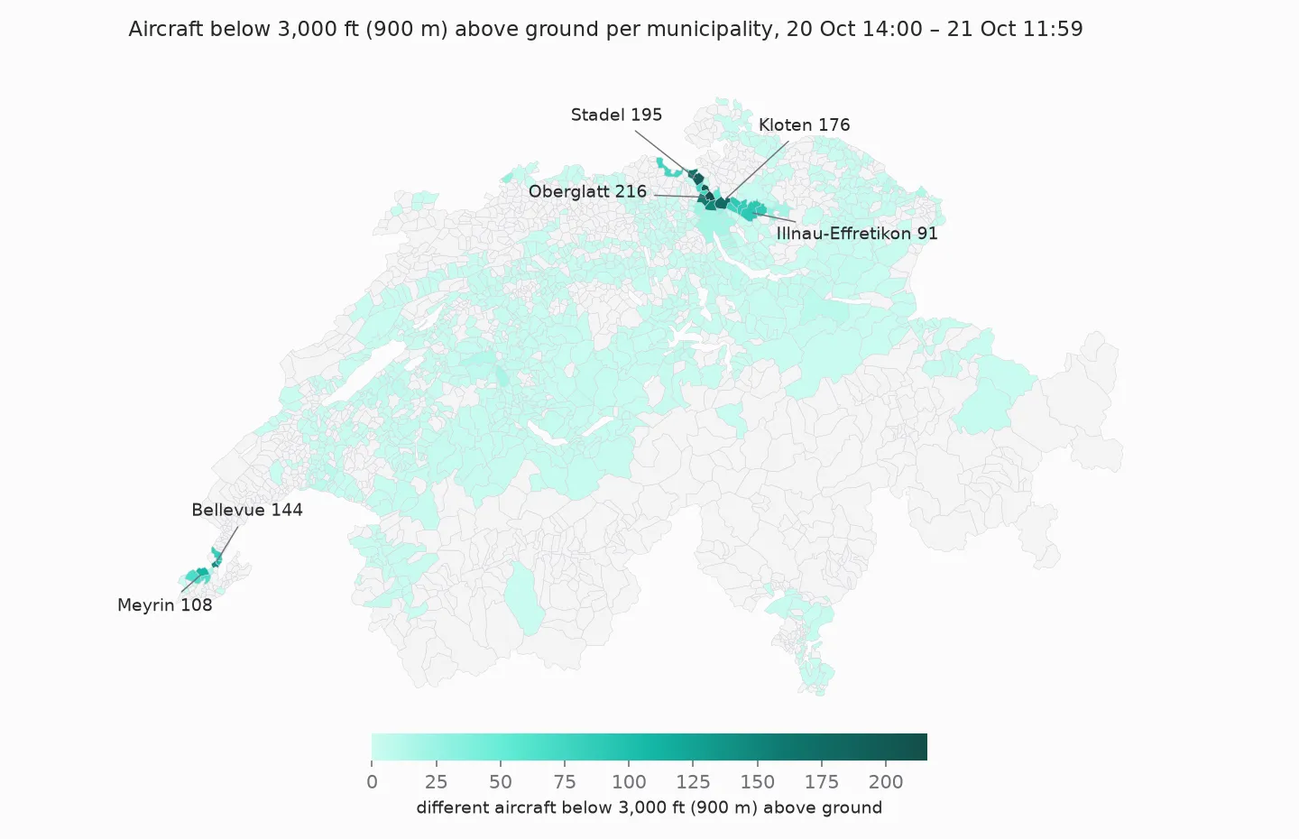
873 municipalities saw at least one aircraft below 3,000 ft, but only a few saw many. The top of the list:

Municipality	Canton	Aircraft < 3,000 ft (900 m)	Residents	Aircraft per km²	Aircraft per 1,000 residents
Oberglatt	ZH	216	7,741	26.2	27.9
Höri	ZH	204	3,676	42.6	55.5
Stadel	ZH	195	2,500	15.1	78.0
Kloten	ZH	176	22,017	9.2	8.0
Weiach	ZH	165	2,133	17.2	77.4
Niederhasli	ZH	157	9,842	13.9	16.0
Rümlang	ZH	148	8,363	11.9	17.7
Bellevue	GE	144	4,111	33.0	35.0
Meyrin	GE	108	27,380	10.9	3.9
Genthod	GE	104	2,814	36.2	37.0

The order depends on what you divide by. In absolute numbers, Oberglatt is first. Per km², it’s Höri, a small municipality right under the approach to runway 14. Per resident, it’s Stadel and Weiach, two villages with just over 2,000 residents each, where almost every approach from the north passes overhead. The city of Zurich, by comparison, had 18 aircraft below 3,000 ft for 440,935 residents.

None of these normalisations is “correct”. Per km² says how often the sky above a place is busy, and per resident how much noise there is per person. Neither says how loud it was – an A220 and a Boeing 777 both count as one aircraft.

The runway decides who

Why Stadel and Weiach, and not the villages east of the airport? Because of the time window. Zurich switches its runway configuration with the time of day, the day of the week and the wind. The airport describes three standard concepts: approaches from the south on runway 34 early in the morning, from the north on runway 14 during the day, and from the east on runway 28 in the evening.

My data shows exactly that, plus one deviation:

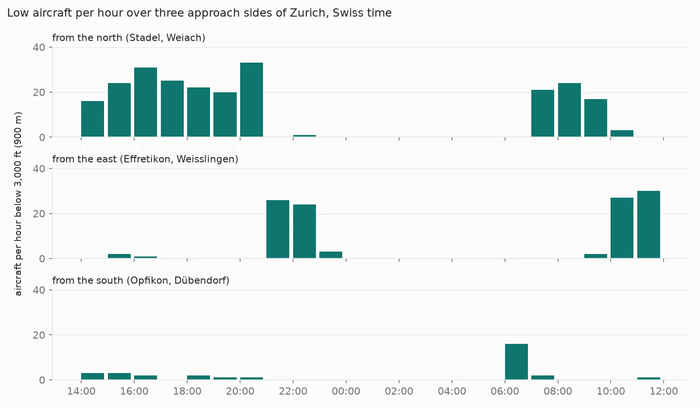
• Tuesday afternoon until 21:00: approaches from the north. Stadel and Weiach see 16 to 33 low aircraft per hour.
• From 21:00: approaches from the east, over Effretikon and Weisslingen. That matches the evening concept on weekdays.
• After 23:00: a few stragglers, and from midnight to 06:00 nothing. That’s the night curfew.
• Wednesday 06:00: 16 aircraft from the south, over Opfikon and Dübendorf, for one hour – the early morning concept on weekdays.
• From 07:00: from the north again.
• From about 10:00: from the east again. That’s not the usual daytime concept, and my position data doesn’t say why. Wind is the usual reason, and a later part of the series compares runways and wind.

So this ranking is a snapshot of a Tuesday and a Wednesday. With a week of bise (a north-easterly wind), other municipalities would be at the top.

People under the tracks

Municipalities are coarse. Kloten has 22,017 residents, but not all of them live under the runway axis. The BFS publishes the population per 100-metre cell, in Swiss coordinates (LV95, metres east and north). In LV95, “within 500 metres” is plain Pythagoras, and swisstopo publishes approximate formulas for the conversion from WGS84 – no extra library needed.

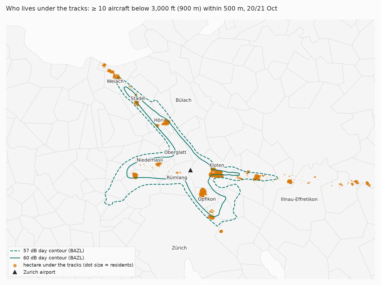
The question: for every inhabited hectare within 30 km of the airport, how many different aircraft passed within 500 metres horizontally, below 3,000 ft (about 900 m) above ground? I call a hectare “under the tracks” if it’s at least 10.

tree = shapely.STRtree(shapely.points(grid_zh["e"], grid_zh["n"]))      # 51,946 inhabited hectares
i, j = tree.query(shapely.points(near["e"], near["n"]), predicate="dwithin", distance=500)
count = (pd.DataFrame({"icao24": near["icao24"].to_numpy()[i], "cell": j})
         .groupby("cell")["icao24"].nunique())
under = grid_zh.iloc[count.index].assign(aircraft=count.to_numpy()).query("aircraft >= 10")

About 31,000 people – 30,923 – live in 705 hectares under the tracks. The busiest hectare saw 93 aircraft. For scale: about 2.1 million people live within 30 km of the airport.

Both thresholds, 10 aircraft and 500 metres, are my choice. With other values the number changes; what stays is where the cells lie.

Compared with the official contours

The BAZL publishes noise contours for Zurich airport: lines of equal noise exposure, calculated, not measured. For residential zones, the Noise Abatement Ordinance sets a planning value of 57 dB and an impact threshold of 60 dB during the day (06–22 h). The contours in the cadastre are valid from 3 July 2015.

	Residents inside the contour	Of those under the tracks
57 dB day	116,183	25,443
60 dB day	48,824	17,765

Of the 30,923 people under the tracks, 25,443 live inside the 57 dB contour and 5,480 outside. On the map you can see where: in a line east of the airport, towards Illnau-Effretikon, and north of the contour’s tip near Weiach. Both are approach paths, and in my window both were busy. The east approach was even in use on a Wednesday morning, when it usually isn’t.

That’s no contradiction. The contours describe noise exposure for an operating scenario, and they weigh loudness and time of day. My count says only how often aircraft were low nearby, in 22 hours. Someone under the approach to runway 28, 10 km from the threshold, hears every aircraft – but each one less loudly than in Kloten.

A broken link along the way

When I reran the notebook for this post, the population grid didn’t load: the BFS had moved the hectare data on data.geo.admin.ch to a new collection, ch.bfs.statistik-bevoelkerung_haushalte. The old URL now returns 404. The new files have a different column for the population (BBTOT). And they make one detail explicit that I hadn’t handled before: people without a geocodable address are counted in a “collective hectare” at the centre of their municipality, marked with NOLOC = 1. Nationwide, these are 53,619 people in 2024. A separate table lists them, and I now subtract them, because they don’t actually live in that hectare.

The course notebook is updated. The licence changed too: the hectare data is now published under opendata.swiss “terms by” – open use with source.

What I take from this

The positions answer “where were aircraft low, and how often” well – and only for the time they cover. Who is overflown depends on the runway configuration, and that changes several times a day. Twenty-two hours are enough to see the patterns, and not enough to rank municipalities for a year.

The count and the official contours largely agree on where the burden lies: four in five of the people under the tracks live inside the 57 dB line. The other fifth lives on approach paths where aircraft are frequent but further from the runway – a fact the position data shows, and the contours, which are calculated for an operating scenario and weigh loudness, don’t.

What’s next

The next part goes down to the ground at Kloten: the weather measured at the airport by MeteoSwiss, and what it has to do with the flights.

Data source

Flight data: The OpenSky Network – Matthias Schäfer, Martin Strohmeier, Vincent Lenders, Ivan Martinovic and Matthias Wilhelm. “Bringing Up OpenSky: A Large-scale ADS-B Sensor Network for Research”. In Proceedings of the 13th IEEE/ACM International Symposium on Information Processing in Sensor Networks (IPSN), pages 83–94, April 2014. doi:10.1109/IPSN.2014.6846743

Municipality boundaries: Federal Statistical Office (BFS), generalised municipality boundaries gg25, as of 1 January 2025. Population per municipality: BFS STATPOP, permanent resident population on 31 December 2025. Population per hectare: BFS STATPOP 2024, via data.geo.admin.ch. Noise contours: BAZL, noise exposure cadastre of Zurich airport (valid from 3 July 2015), via the WFS of the Canton of Zurich. Airport position: OurAirports, public domain.

Useful Links

Geodata and population

• BFS: Generalised municipality boundaries – gg25, with a data description
• BFS: Population and households from 2010 – the hectare data, with the data description that explains NOLOC
• swisstopo: approximate formulas WGS84 ↔ LV95 – the conversion without an extra library

Noise

• BAZL: noise exposure cadastre – the official contours of the national airports
• Noise Abatement Ordinance (LSV, SR 814.41) – annex 5: exposure limits for civil aerodromes
• Flughafen Zürich: operating concepts – which runway when

Related posts

• Part 5 – silver – where altitude_ft and the flight phases come from
• Part 10 – analysis – take-offs and landings in Zurich over the same days
• Part 11 – rail – the previous part: plane or train