Live Flight Data Step by Step - Part 16 - The app

Every part so far ended in a notebook: code, a table, a chart. That’s the right tool while you’re asking questions. It’s the wrong tool for someone who just wants to look at the answer – or at the aircraft over Switzerland right now.

The course has two answers to that. A notebook that runs as an app, and a live map. Part 6 showed the map for a moment. This part shows how both are built.

A notebook as a dashboard

marimo notebooks are plain Python files, and part 2 mentioned that they can run as apps. Notebook 20 uses that. The same file opens in two ways:

uv run marimo edit solutions/20_dashboard.py   # the notebook: code, text, checks
uv run marimo run solutions/20_dashboard.py    # the app: only outputs and controls

In marimo run the code is hidden (marimo: apps). The dropdown still works: picking another airport reruns every cell that reads it, as in the notebook. The notebook knows which mode it’s in, and hides its own explanations in the app:

IN_APP = mo.app_meta().mode == "run"

mo.md("## TODO 20.1 – Three KPIs ...") if not IN_APP else None

The page itself is four pieces: three numbers, an airport dropdown, a chart of departures and arrivals per 15 minutes, and a table. And a refresh:

refresh = mo.ui.refresh(options=["1m", "5m"], default_interval="1m", label="Refresh")

refresh                    # reading it makes this cell rerun every minute
con = fl.snapshot()        # a fresh copy of flights.duckdb

Every minute the dashboard takes a new copy of the database and everything below recomputes. Why a copy, and not the database itself, is the main story of the second app.

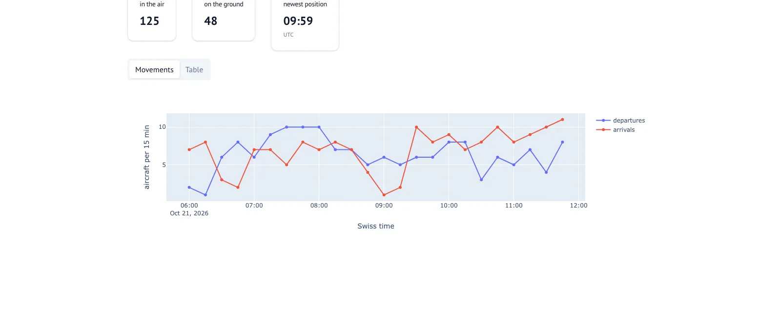
Here it runs on the data of the series, so “now” is the end of the window, 21 October 09:59 UTC, and the chart shows the last six hours before it.

The live map

The second app is the one from part 6: a Dash application with a Leaflet map, about 1,500 lines in app/app.py. One command starts it:

uv run start.py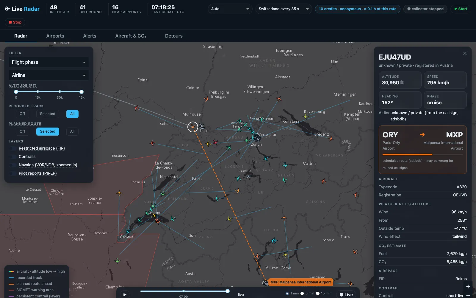

This is the map live, on a Wednesday morning in November. The panel on the right is one aircraft: an easyJet A320 from Paris-Orly to Milan Malpensa, with the weather at its altitude and its CO₂ estimate. Two things in the picture are worth a second look:

• “unknown / private” as the airline. The callsign starts with EJU, easyJet Europe. The airline list of the course comes from OpenFlights, and it has EZY for easyJet, but not EJU or EZS. The map tells the truth about its data, not about the aircraft.
• 10 credits in the header. When I started the app that morning, OpenSky’s anonymous allowance for my internet connection was already down to 12 – I don’t know what used the rest. Below 20 credits the collector pauses for half an hour, so in 37 minutes the map got three snapshots, and its tracks are straight lines between them.

One process owns the database

In the DuckDB version the course uses (1.5), one process at a time can open a database file for writing, and other processes then can’t open it, not even to read (DuckDB: concurrency). A notebook that tries gets Could not set lock on file.

So the app is not only the map. It’s the process that owns flights.duckdb, and it does everything that writes to it, in background threads:

• collector: one OpenSky call every 35 seconds into bronze, then silver – the code of parts 2 to 5;
• enrichment: the analyses of parts 7 to 15 as jobs, each on its own rhythm – weather, routes, CO₂, contrails, runways, go-arounds, holdings.

Inside one process, DuckDB is happy with many threads, as long as each has its own cursor (DuckDB Python API). Every query of the map gets one:

def utc_cursor(con):
    """A cursor is a new connection: it does NOT inherit SET TimeZone – without this, timestamps shift by 1–2 h."""
    cur = con.cursor()
    cur.execute("SET TimeZone = 'UTC'")
    return cur

A cursor is a new connection to the same database, with its own session settings. I tested it: the connection is set to UTC, a cursor of it reports Europe/Zurich, the time zone of my laptop. Without the SET, every timestamp the map reads would be one or two hours off – the trap of part 2, one level deeper.

The notebooks never touch the app’s file. fl.snapshot() copies it, and they analyse the copy. That’s why notebook 20 reads a copy every minute: the original belongs to the app.

Only what you see

Over Switzerland, my 22 hours had 100 aircraft per snapshot in the median and at most 178. With the course’s archive, the app can also show the whole world, about 13,000. Drawing 13,000 rotated symbols with tracks every 15 seconds makes a browser slow. So the map asks only for the aircraft inside the visible part of the map, draws tracks only for the 500 closest to the centre, and switches to plain dots above 3,000 aircraft in view.

The positions themselves are read once per refresh into memory and shared by everyone who has the page open. A click on an aircraft reads from there, not from the database.

A click on an aircraft

The panel on the right collects what the pipeline knows about one aircraft: type and registration from the OpenSky aircraft database, the weather at its altitude, the CO₂ estimate of part 8, whether it leaves a contrail (part 9), and its route.

The route comes from adsbdb, like in part 7 – with the lesson from there. Callsigns are reused, and adsbdb sometimes answers with an old route. Before the map draws the planned route, it checks it against the aircraft’s position:

gcd, via = haversine_km(*o, *d), haversine_km(*o, *ac) + haversine_km(*ac, *d)
if via > 1.3 * gcd + 150:
    return f"it is {via - gcd:,.0f} km off the direct line"

If the aircraft is far off the line between origin and destination, or flies away from the destination, the map says why and doesn’t draw the route.

A photo comes from planespotters.net, but only if you put a contact address into .env: the app sends it along with every request, asks for at most 30 aircraft near airports every 30 minutes plus the one you click, and shows the photographer’s name and a link to the photo page. Without a contact, it shows no photos.

The time slider

Silver keeps every position, so the map can show any moment of the past: the same query as gold.current_positions, with an older “now”.

SELECT ... FROM silver.flights f LEFT JOIN silver.airlines a USING (airline_icao)
WHERE f.snapshot_time BETWEEN TIMESTAMP '{ts}' - INTERVAL 2 MINUTE AND TIMESTAMP '{ts}'
QUALIFY ROW_NUMBER() OVER (PARTITION BY f.icao24 ORDER BY f.snapshot_time DESC) = 1

The play button moves “now” forward one, five or fifteen minutes per step. Here’s 20 October at 14:30 Swiss time, in the middle of the 37 minutes of part 10:

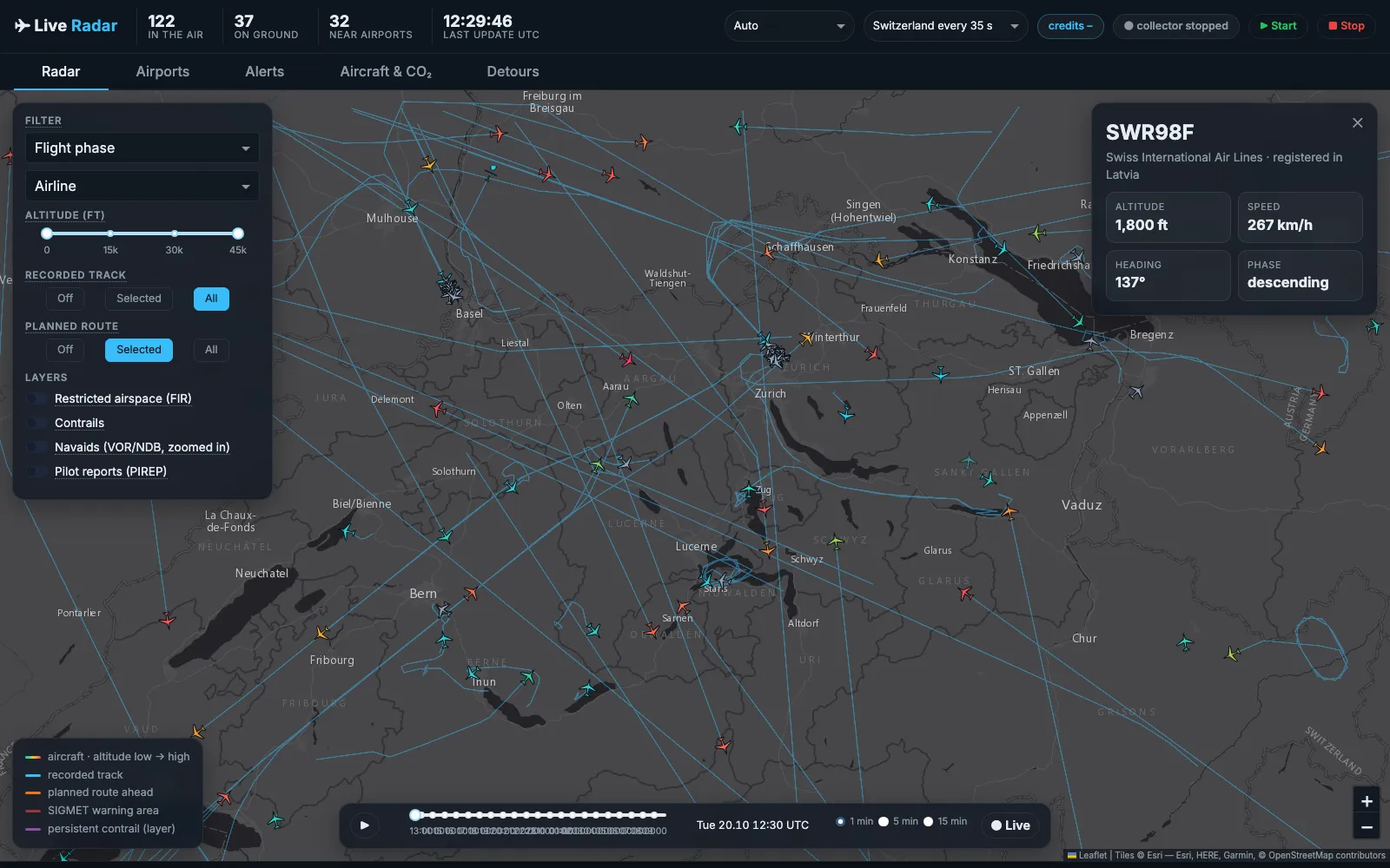
12:30 UTC is 14:30 in Zurich. SWR98F is on its approach, 1,800 ft and descending. The cluster at the airport is aircraft on the ground; between 14:14 and 14:51 no airliner took off (part 10). The map shows the fault. It doesn’t explain it.

The tabs

Behind the map are four tabs with the analyses as tables: Airports (runway in use, weather reports and forecasts, the busiest radio beacons), Alerts (aircraft in a SIGMET warning area, emergency squawks, go-arounds, holdings), Aircraft & CO₂, and Detours (flown route against the great circle, part 7).

The Alerts tab shows the go-around and holding detectors of part 15 – live, without anyone checking each case. After part 15 I’d read every go-around there as “maybe an echo”.

What doesn’t work so well

• Live weather on a live map only. The weather jobs fetch the reports and forecasts of now. That’s right for the live map, and wrong for the time slider: on 20 October it shows today’s METAR.
• Credits. Without an OpenSky account, you get 400 credits a day (OpenSky REST API, and part 3). One call for Switzerland costs one, so at 35 seconds the collector runs for about four hours. The app shows the credits left in the header. With a free account and API client, it’s 4,000.
• One file, 1,500 lines. app.py grew with every part of the series. The map layers are in their own module, radar.py. The callbacks aren’t, and the file is longer than I’d like.
• A development server. app.run() starts Flask’s development server. For one person on a laptop that’s fine. To share the map with others, it would need a proper server, and the OpenSky terms would need a look first.

What’s next

The next part is the last one: a look back at the series – what worked, what didn’t, what I’d do differently, and what’s left to analyse. And the link to the code.

Data sources

Flight data: The OpenSky Network – Matthias Schäfer, Martin Strohmeier, Vincent Lenders, Ivan Martinovic and Matthias Wilhelm. “Bringing Up OpenSky: A Large-scale ADS-B Sensor Network for Research”. In Proceedings of the 13th IEEE/ACM International Symposium on Information Processing in Sensor Networks (IPSN), pages 83–94, April 2014. doi:10.1109/IPSN.2014.6846743

In the screenshots: routes from adsbdb, weather reports from aviationweather.gov, airports from OurAirports (public domain), map tiles © Esri, HERE, Garmin, © OpenStreetMap contributors.

Useful Links

• marimo: run notebooks as apps
• Dash and Dash Leaflet
• DuckDB: concurrency – one writing process

Related posts

• Part 6 – gold and the first look at the map
• Part 7 – routes, and why almost a quarter are wrong
• Part 15 – holdings, go-arounds and echoes – the previous part